Running A Backtest
In this example we will demonstrate how to run a backtest for a simple algo example
Loading the data bundle
[95]:
import os

import warnings
warnings.filterwarnings('ignore')

os.environ['ZIPLINE_ROOT'] = os.path.join(os.getcwd(), '.zipline')

os.listdir(os.environ['ZIPLINE_ROOT'])

os.environ['ZIPLINE_TRADER_CONFIG'] = os.path.join(os.getcwd(), "./zipline-trader.yaml")

with open(os.environ['ZIPLINE_TRADER_CONFIG'], 'r') as f:
    data = f.read()
    print(data[:20])

import zipline
from zipline.data import bundles

bundle_name = 'alpaca_api'
bundle_data = bundles.load(bundle_name)
from zipline.pipeline.loaders import USEquityPricingLoader
from zipline.utils.calendars import get_calendar
from zipline.pipeline.data import USEquityPricing
from zipline.data.data_portal import DataPortal

import pandas as pd

# Set the dataloader
pricing_loader = USEquityPricingLoader.without_fx(bundle_data.equity_daily_bar_reader, bundle_data.adjustment_reader)


# Define the function for the get_loader parameter
def choose_loader(column):
    if column not in USEquityPricing.columns:
        raise Exception('Column not in USEquityPricing')
    return pricing_loader

# Set the trading calendar
trading_calendar = get_calendar('NYSE')

start_date = pd.Timestamp('2019-07-05', tz='utc')
end_date = pd.Timestamp('2020-11-13', tz='utc')

# Create a data portal
data_portal = DataPortal(bundle_data.asset_finder,
                         trading_calendar = trading_calendar,
                         first_trading_day = start_date,
                         equity_daily_reader = bundle_data.equity_daily_bar_reader,
                         adjustment_reader = bundle_data.adjustment_reader)
[96]:
import dateutil.parser
from os.path import join, exists
import pandas as pd
import pandas_datareader.data as yahoo_reader
import yaml

import numpy as np


def get_benchmark(symbol=None, start = None, end = None, other_file_path=None):
    bm = yahoo_reader.DataReader(symbol,
                                 'yahoo',
                                 pd.Timestamp(start),
                                 pd.Timestamp(end))['Close']
    bm.index = bm.index.tz_localize('UTC')
    return bm.pct_change(periods=1).fillna(0)
[97]:
from zipline.api import order_target, record, symbol
import matplotlib.pyplot as plt
def initialize(context):
context.equity = bundle_data.asset_finder.lookup_symbol("AMZN", end_date)
def handle_data(context, data):
order_target(context.equity, 100)
def before_trading_start(context, data):
pass
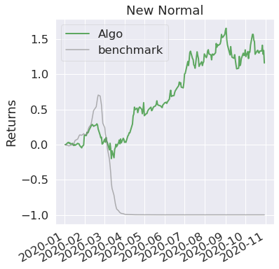
def analyze(context, perf):
ax1 = plt.subplot(211)
perf.portfolio_value.plot(ax=ax1)
ax2 = plt.subplot(212, sharex=ax1)
perf.sym.plot(ax=ax2, color='r')
plt.gcf().set_size_inches(18, 8)
plt.legend(['Algo', 'Benchmark'])
plt.ylabel("Returns", color='black', size=25)
[98]:
import pandas as pd
from datetime import datetime
import pytz
from zipline import run_algorithm
start = pd.Timestamp(datetime(2020, 1, 1, tzinfo=pytz.UTC))
end = pd.Timestamp(datetime(2020, 11, 1, tzinfo=pytz.UTC))
r = run_algorithm(start=start,
end=end,
initialize=initialize,
capital_base=100000,
handle_data=handle_data,
benchmark_returns=get_benchmark(symbol="SPY",
start=start.date().isoformat(),
end=end.date().isoformat()),
bundle='alpaca_api',
broker=None,
state_filename="./demo.state",
trading_calendar=trading_calendar,
before_trading_start=before_trading_start,
# analyze=analyze,
data_frequency='daily'
)
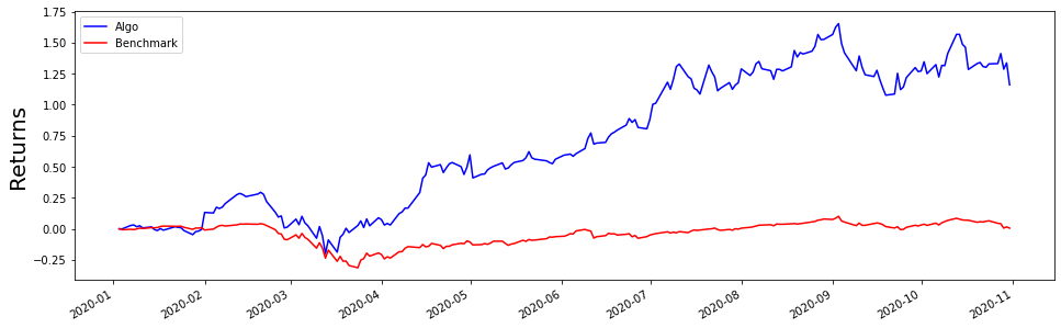
fig, axes = plt.subplots(1, 1, figsize=(16, 5), sharex=True)
r.algorithm_period_return.plot(color='blue')
r.benchmark_period_return.plot(color='red')
plt.legend(['Algo', 'Benchmark'])
plt.ylabel("Returns", color='black', size=20)
[98]:
Text(0, 0.5, 'Returns')
Using Pyfolio to analyze your results
[99]:
import pyfolio as pf
returns, positions, transactions = pf.utils.extract_rets_pos_txn_from_zipline(r)
benchmark_returns = r.benchmark_period_return
[100]:
import empyrical
print("returns sharp ratio: {}".format(empyrical.sharpe_ratio(returns)))  # how much is it sensative to divergance. the higher the better
print("bencmark sharp ratio: {}".format(empyrical.sharpe_ratio(benchmark_returns)))
print("beta ratio: {}".format(empyrical.beta(returns, benchmark_returns))) # how much correlation between algo to benchmark. we want it to be clsoe to zero
print("alpha ratio: {}".format(empyrical.alpha(returns, benchmark_returns)))
returns sharp ratio: 1.7147226500268884
bencmark sharp ratio: -6.584559370521319
beta ratio: -0.010817530431739008
alpha ratio: 1.829456229577063
[101]:
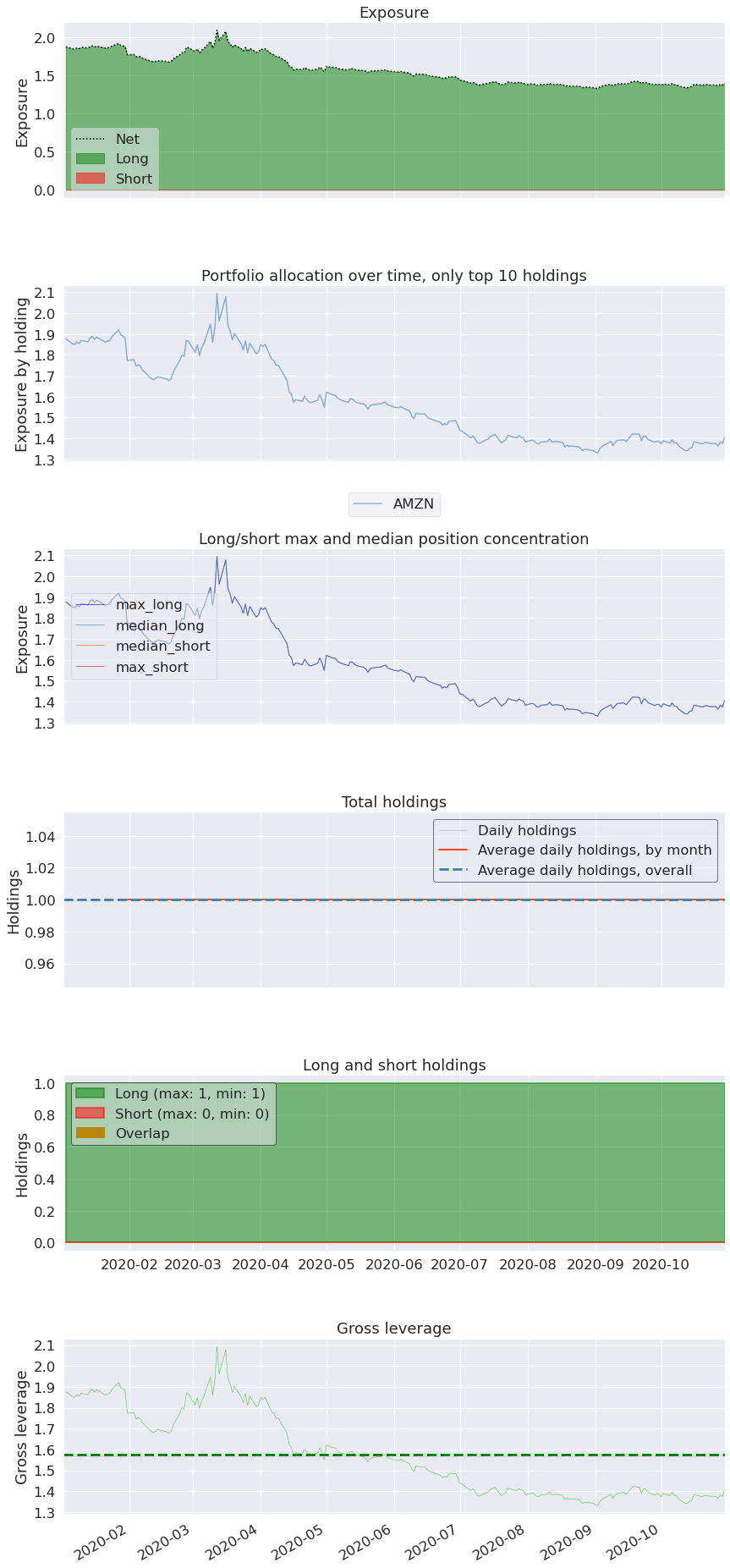
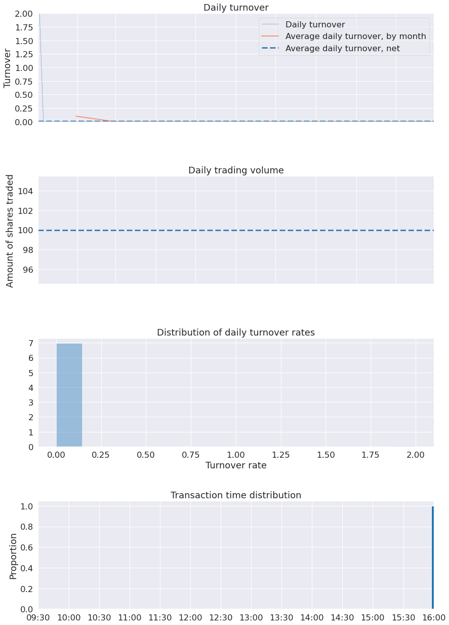
pf.create_position_tear_sheet(returns, positions=positions, transactions=transactions)
| Top 10 long positions of all time | max |
|---|---|
| sid | |
| AMZN | 209.44% |
| Top 10 short positions of all time | max |
|---|---|
| sid |
| Top 10 positions of all time | max |
|---|---|
| sid | |
| AMZN | 209.44% |

[102]:
pf.create_returns_tear_sheet(returns,
                             positions=positions,
                             transactions=transactions,
                             benchmark_rets=benchmark_returns)
| Start date | 2020-01-02 | |
|---|---|---|
| End date | 2020-10-30 | |
| Total months | 10 | |
| Backtest | ||
| Annual return | 150.903% | |
| Cumulative returns | 116.026% | |
| Annual volatility | 66.542% | |
| Sharpe ratio | 1.71 | |
| Calmar ratio | 3.95 | |
| Stability | 0.87 | |
| Max drawdown | -38.166% | |
| Omega ratio | 1.35 | |
| Sortino ratio | 2.67 | |
| Skew | 0.13 | |
| Kurtosis | 1.98 | |
| Tail ratio | 1.17 | |
| Daily value at risk | -7.931% | |
| Gross leverage | 1.57 | |
| Daily turnover | 0.953% | |
| Alpha | 1.83 | |
| Beta | -0.01 | |
| Worst drawdown periods | Net drawdown in % | Peak date | Valley date | Recovery date | Duration |
|---|---|---|---|---|---|
| 0 | 38.17 | 2020-02-19 | 2020-03-12 | 2020-04-14 | 40 |
| 1 | 21.73 | 2020-09-02 | 2020-09-18 | NaT | NaN |
| 2 | 11.63 | 2020-04-30 | 2020-05-01 | 2020-05-20 | 15 |
| 3 | 10.39 | 2020-07-10 | 2020-07-17 | 2020-08-05 | 19 |
| 4 | 7.56 | 2020-01-07 | 2020-01-27 | 2020-01-31 | 19 |
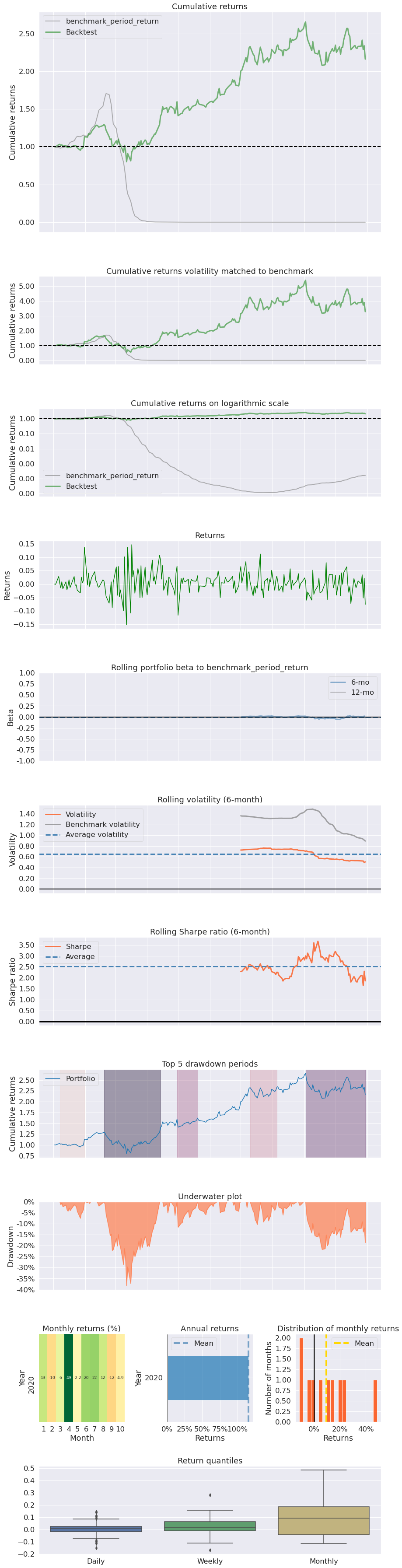
[103]:
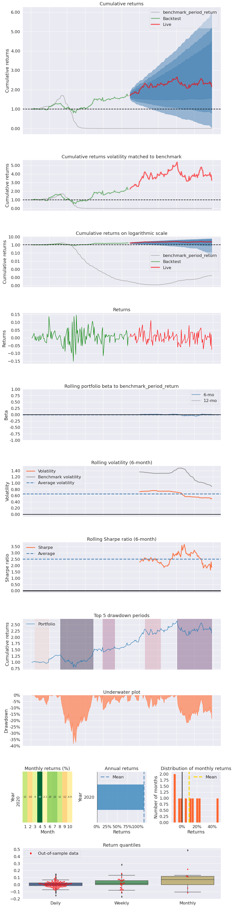
pf.create_full_tear_sheet(returns,
                          positions=positions,
                          transactions=transactions,
                          live_start_date="2020-06-13",
                          round_trips=True,
                          benchmark_rets=benchmark_returns)
| Start date | 2020-01-02 | |||
|---|---|---|---|---|
| End date | 2020-10-30 | |||
| In-sample months | 5 | |||
| Out-of-sample months | 4 | |||
| All | In-sample | Out-of-sample | ||
| Annual return | 150.903% | 222.617% | 87.764% | |
| Cumulative returns | 116.026% | 69.084% | 27.763% | |
| Annual volatility | 66.542% | 75.493% | 54.733% | |
| Sharpe ratio | 1.71 | 1.93 | 1.42 | |
| Calmar ratio | 3.95 | 5.83 | 4.04 | |
| Stability | 0.87 | 0.63 | 0.40 | |
| Max drawdown | -38.166% | -38.166% | -21.734% | |
| Omega ratio | 1.35 | 1.42 | 1.26 | |
| Sortino ratio | 2.67 | 3.01 | 2.22 | |
| Skew | 0.13 | 0.05 | 0.23 | |
| Kurtosis | 1.98 | 1.85 | 0.37 | |
| Tail ratio | 1.17 | 1.24 | 1.10 | |
| Daily value at risk | -7.931% | -8.933% | -6.587% | |
| Gross leverage | 1.57 | 1.73 | 1.40 | |
| Daily turnover | 0.953% | 1.787% | 0.0% | |
| Alpha | 1.83 | 3.35 | 1.42 | |
| Beta | -0.01 | 0.00 | -0.02 | |
| Worst drawdown periods | Net drawdown in % | Peak date | Valley date | Recovery date | Duration |
|---|---|---|---|---|---|
| 0 | 38.17 | 2020-02-19 | 2020-03-12 | 2020-04-14 | 40 |
| 1 | 21.73 | 2020-09-02 | 2020-09-18 | NaT | NaN |
| 2 | 11.63 | 2020-04-30 | 2020-05-01 | 2020-05-20 | 15 |
| 3 | 10.39 | 2020-07-10 | 2020-07-17 | 2020-08-05 | 19 |
| 4 | 7.56 | 2020-01-07 | 2020-01-27 | 2020-01-31 | 19 |
| Stress Events | mean | min | max |
|---|---|---|---|
| New Normal | 0.45% | -15.20% | 14.70% |
| Top 10 long positions of all time | max |
|---|---|
| sid | |
| AMZN | 209.44% |
| Top 10 short positions of all time | max |
|---|---|
| sid |
| Top 10 positions of all time | max |
|---|---|
| sid | |
| AMZN | 209.44% |