Using Alphalens

In this example we will demonstrate how to create a simple pipeline that uses a factor and then analyze it using alphalens.

Loading the data bundle

import warnings
warnings.filterwarnings('ignore')

import os
import pandas as pd
from datetime import timedelta

os.environ['ZIPLINE_ROOT'] = os.path.join(os.getcwd(), '.zipline')
os.listdir(os.environ['ZIPLINE_ROOT'])

os.environ['ZIPLINE_TRADER_CONFIG'] = os.path.join(os.getcwd(), "./zipline-trader.yaml")

with open(os.environ['ZIPLINE_TRADER_CONFIG'], 'r') as f:
    data = f.read()
    print(data[:20])
import zipline
from zipline.data import bundles

from zipline.utils.calendars import get_calendar
from zipline.pipeline.data import USEquityPricing
from zipline.pipeline.factors import CustomFactor
from zipline.research.utils import get_pricing, create_data_portal, create_pipeline_engine

# Set the trading calendar
trading_calendar = get_calendar('NYSE')
bundle_name = 'alpaca_api'
start_date = pd.Timestamp('2015-12-31', tz='utc')
pipeline_start_date = start_date + timedelta(days=365*2+10)
end_date = pd.Timestamp('2020-12-28', tz='utc')
data_portal = create_data_portal(bundle_name, trading_calendar, start_date)

Creating the Pipeline Engine

engine = create_pipeline_engine(bundle_name)

Let’s create our custom factor

This is a factor that runs a linear regression over one year of stock log returns and calculates a “slope” as our factor.

from zipline.pipeline.factors import CustomFactor, Returns
from zipline.pipeline.data import USEquityPricing

class YearlyReturns(CustomFactor):
    inputs = [USEquityPricing.close]
    window_length = 252
    def compute(self, today, assets, out, prices):
        start = self.window_length
        out[:] = (prices[-1] - prices[-start])/prices[-start]

Our Pipeline

from zipline.pipeline.domain import US_EQUITIES
from zipline.pipeline.factors import AverageDollarVolume
from zipline.pipeline import Pipeline
from zipline.pipeline.classifiers.custom.sector import ZiplineTraderSector, SECTOR_LABELS

universe = USEquityPricing
universe = AverageDollarVolume(window_length = 5)

pipeline = Pipeline(
    columns = {
            'MyFactor' : YearlyReturns(),
#             'Returns': Returns(window_length=252),  # same as YearlyRetruns
            'Sector' : ZiplineTraderSector()
    }, domain=US_EQUITIES
)

Run the Pipeline

# Run our pipeline for the given start and end dates
factors = engine.run_pipeline(pipeline, pipeline_start_date, end_date)

factors.head()

		MyFactor	Sector
2018-01-09 00:00:00+00:00	Equity(0 [A])	0.455036	1
	Equity(1 [AAL])	0.118720	11
	Equity(2 [ABC])	0.133466	7
	Equity(3 [ABMD])	0.774400	7
	Equity(4 [ADP])	0.150161	10

Data preparation

Alphalens input consists of two type of information: the factor values for the time period under analysis and the historical assets prices (or returns). Alphalens doesn’t need to know how the factor was computed, the historical factor values are enough. This is interesting because we can use the tool to evaluate factors for which we have the data but not the implementation details.

Alphalens requires that factor and price data follows a specific format and it provides an utility function, get_clean_factor_and_forward_returns, that accepts factor data, price data and optionally a group information (for example the sector groups, useful to perform sector specific analysis) and returns the data suitably formatted for Alphalens.

asset_list = factors.index.levels[1].unique()

prices = get_pricing(
        data_portal,
        trading_calendar,
        asset_list,
        pipeline_start_date,
        end_date)
prices.head()

	Equity(0 [A])	Equity(1 [AAL])	Equity(2 [ABC])	Equity(3 [ABMD])	Equity(4 [ADP])	Equity(5 [AEE])	Equity(6 [AES])	Equity(7 [AJG])	Equity(8 [ALB])	Equity(9 [ALK])	...	Equity(495 [TWTR])	Equity(496 [UNM])	Equity(497 [UNP])	Equity(498 [UPS])	Equity(499 [VMC])	Equity(500 [VRSK])	Equity(501 [VZ])	Equity(502 [WBA])	Equity(503 [WEC])	Equity(504 [ZTS])
2018-01-10 00:00:00+00:00	70.80	53.78	97.20	208.21	117.66	56.49	10.775	63.575	132.96	72.07	...	24.240	57.520	139.71	129.77	132.39	96.32	51.69	74.06	63.68	73.90
2018-01-11 00:00:00+00:00	70.80	56.18	98.12	210.17	117.18	56.15	10.960	63.390	134.68	74.82	...	24.340	58.210	140.40	133.46	135.18	96.67	52.12	75.36	63.58	74.60
2018-01-12 00:00:00+00:00	71.72	58.22	98.99	215.19	118.39	55.50	11.030	63.875	133.46	73.52	...	25.415	58.600	141.17	134.08	133.97	97.48	51.87	76.03	63.63	75.40
2018-01-16 00:00:00+00:00	71.24	57.73	99.55	218.27	119.38	55.45	10.680	63.410	128.00	71.28	...	24.680	55.530	140.30	132.90	133.67	97.19	51.66	76.03	63.15	75.55
2018-01-17 00:00:00+00:00	72.05	57.91	101.29	224.23	122.05	55.79	10.730	64.040	126.96	70.83	...	24.550	56.355	140.46	134.01	134.58	98.01	51.73	75.78	63.56	76.76

5 rows × 505 columns

import alphalens as al

factor_data = al.utils.get_clean_factor_and_forward_returns(
        factor=factors["MyFactor"],
        prices=prices,
        quantiles=5,
        periods=[1, 5, 10],
        groupby=factors["Sector"],
        binning_by_group=True,
        groupby_labels=SECTOR_LABELS,
    max_loss=0.8)

Dropped 1.5% entries from factor data: 1.5% in forward returns computation and 0.0% in binning phase (set max_loss=0 to see potentially suppressed Exceptions).
max_loss is 80.0%, not exceeded: OK!

factor_data.head(10)

		1D	5D	10D	factor	group	factor_quantile
date	asset
2018-01-10 00:00:00+00:00	Equity(0 [A])	0.000000	0.019492	0.043079	0.491687	Capital Goods	4
	Equity(1 [AAL])	0.044626	0.080141	-0.017851	0.085696	Transportation	2
	Equity(2 [ABC])	0.009465	0.037757	0.073765	0.149593	Health Care	3
	Equity(3 [ABMD])	0.009414	0.084914	0.135200	0.868852	Health Care	5
	Equity(4 [ADP])	-0.004080	0.027707	0.025497	0.162133	Technology	1
	Equity(5 [AEE])	-0.006019	-0.019295	0.004780	0.102944	Public Utilities	3
	Equity(6 [AES])	0.017169	0.070070	0.067285	-0.050309	Basic Industries	1
	Equity(7 [AJG])	-0.002910	0.007000	0.032796	0.213659	Finance	3
	Equity(8 [ALB])	0.012936	-0.113147	-0.120751	0.507343	Basic Industries	5
	Equity(9 [ALK])	0.038157	-0.031636	-0.138754	-0.225000	Transportation	1

Running Alphalens

Once the factor data is ready, running Alphalens analysis is pretty simple and it consists of one function call that generates the factor report (statistical information and plots). Please remember that it is possible to use the help python built-in function to view the details of a function.

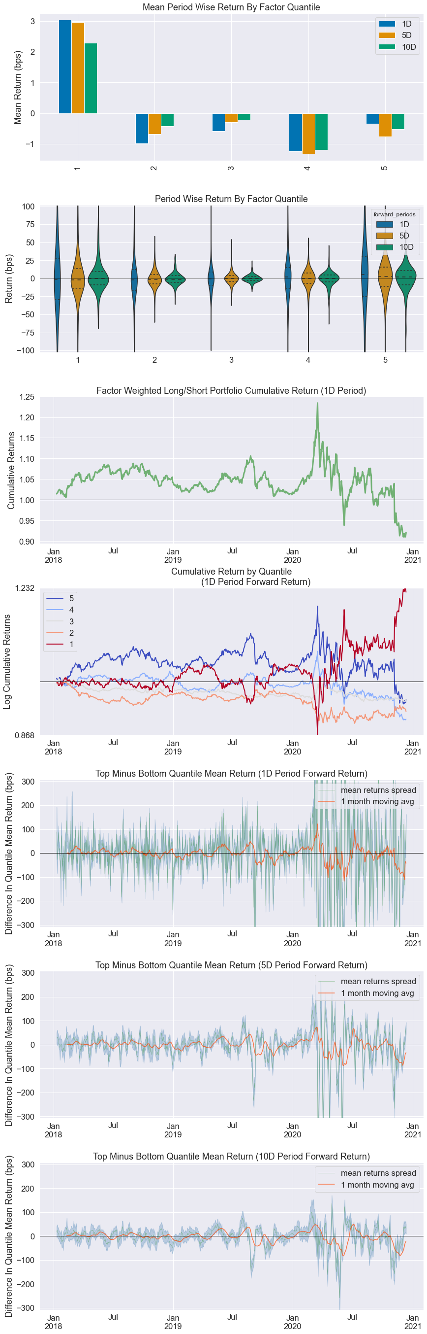
al.tears.create_full_tear_sheet(factor_data, long_short=True, group_neutral=False, by_group=True)

Quantiles Statistics

	min	max	mean	std	count	count %
factor_quantile
1	-0.882437	0.336851	-0.221892	0.173761	77857	20.919291
2	-0.788964	0.440738	-0.049322	0.143953	74322	19.969477
3	-0.671378	0.560727	0.058053	0.144160	70527	18.949804
4	-0.570969	0.765367	0.176418	0.153070	74354	19.978075
5	-0.463738	9.102661	0.436519	0.325251	75118	20.183353

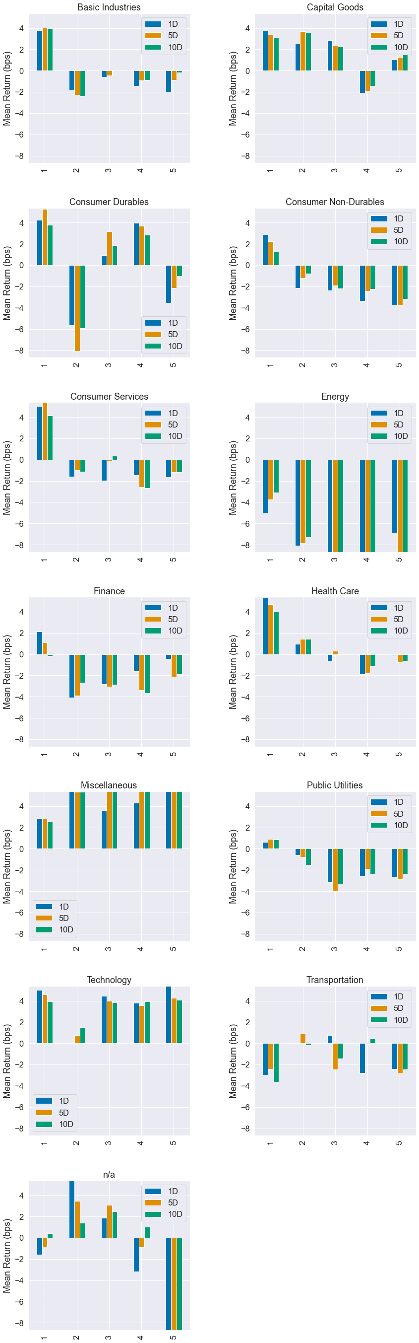
Returns Analysis

	1D	5D	10D
Ann. alpha	0.012	0.007	0.008
beta	-0.236	-0.309	-0.262
Mean Period Wise Return Top Quantile (bps)	-0.345	-0.764	-0.528
Mean Period Wise Return Bottom Quantile (bps)	3.034	2.960	2.288
Mean Period Wise Spread (bps)	-3.380	-3.663	-2.783

<Figure size 432x288 with 0 Axes>

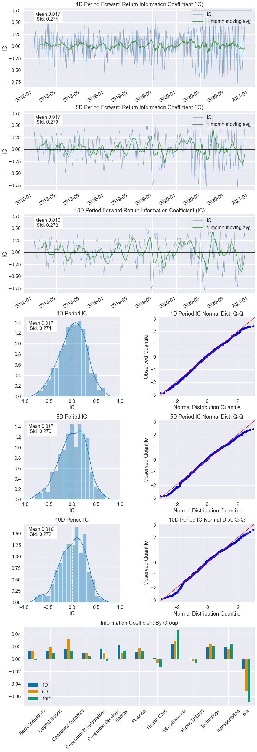
Information Analysis

	1D	5D	10D
IC Mean	0.017	0.017	0.010
IC Std.	0.274	0.279	0.272
Risk-Adjusted IC	0.061	0.060	0.036
t-stat(IC)	1.648	1.640	0.970
p-value(IC)	0.100	0.101	0.332
IC Skew	-0.228	-0.323	-0.357
IC Kurtosis	-0.256	-0.193	-0.076

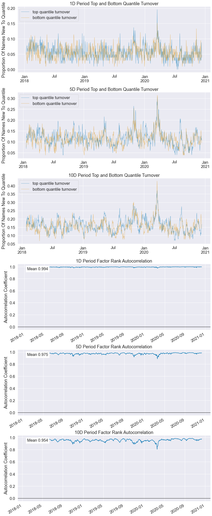
Turnover Analysis

	1D	5D	10D
Quantile 1 Mean Turnover	0.054	0.113	0.155
Quantile 2 Mean Turnover	0.132	0.267	0.354
Quantile 3 Mean Turnover	0.159	0.312	0.408
Quantile 4 Mean Turnover	0.131	0.265	0.353
Quantile 5 Mean Turnover	0.056	0.117	0.162

	1D	5D	10D
Mean Factor Rank Autocorrelation	0.994	0.975	0.954

These reports are also available

al.tears.create_returns_tear_sheet(factor_data,
                                   long_short=True,
                                   group_neutral=False,
                                   by_group=False)

al.tears.create_information_tear_sheet(factor_data,
                                       group_neutral=False,
                                       by_group=False)

al.tears.create_turnover_tear_sheet(factor_data)

al.tears.create_event_returns_tear_sheet(factor_data, prices,
                                         avgretplot=(5, 15),
                                         long_short=True,
                                         group_neutral=False,
                                         std_bar=True,
                                         by_group=False)

Working with Pyfolio

We could use pyfolio to analyze the returns as if it was generated by a backtest, like so

pf_returns, pf_positions, pf_benchmark = \
    al.performance.create_pyfolio_input(factor_data,
                                        period='1D',
                                        capital=100000,
                                        long_short=True,
                                        group_neutral=False,
                                        equal_weight=True,
                                        quantiles=[1,5],
                                        groups=None,
                                        benchmark_period='1D')

import pyfolio as pf
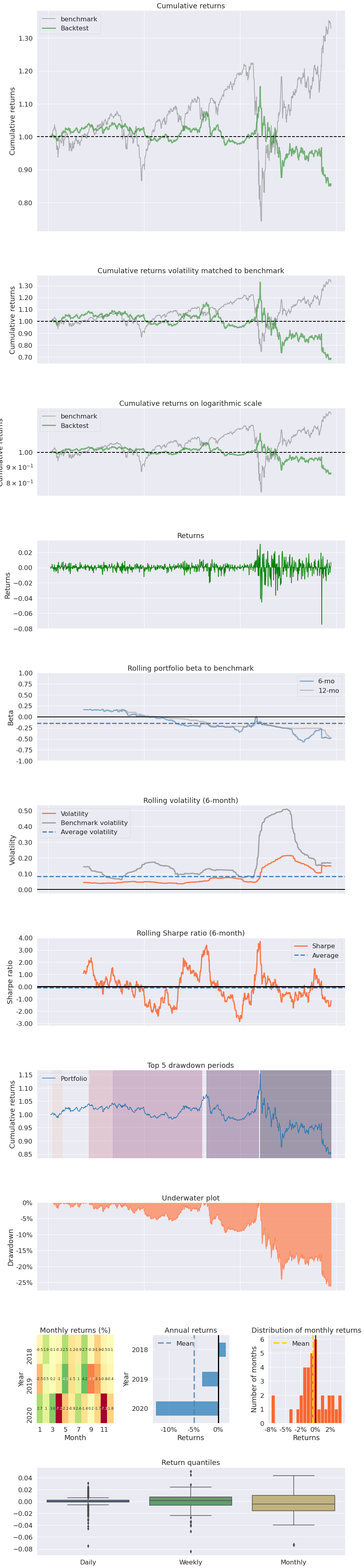
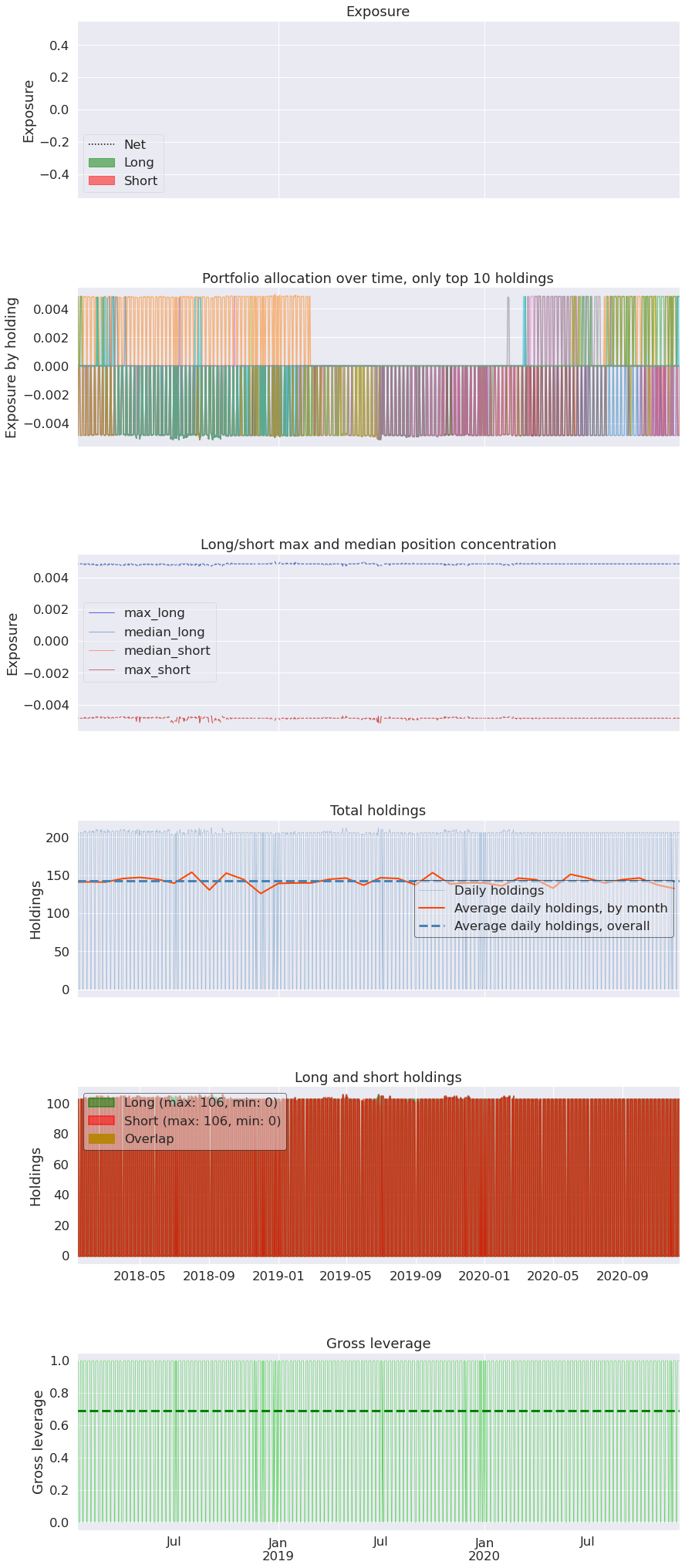
pf.tears.create_full_tear_sheet(pf_returns,
                                positions=pf_positions,
                                benchmark_rets=pf_benchmark,
                                hide_positions=True)

Start date	2018-01-10
End date	2020-12-11
Total months	50
	Backtest
Annual return	-3.584%
Cumulative returns	-14.318%
Annual volatility	10.102%
Sharpe ratio	-0.31
Calmar ratio	-0.14
Stability	0.36
Max drawdown	-26.261%
Omega ratio	0.93
Sortino ratio	-0.39
Skew	-2.46
Kurtosis	25.59
Tail ratio	0.84
Daily value at risk	-1.285%
Gross leverage	0.69
Alpha	-0.01
Beta	-0.23

Worst drawdown periods	Net drawdown in %	Peak date	Valley date	Recovery date	Duration
0	26.26	2020-03-17	2020-12-09	NaT	NaN
1	9.46	2019-08-26	2019-11-04	2020-03-11	143
2	5.86	2018-09-03	2019-04-17	2019-08-08	244
3	2.92	2018-06-04	2018-07-30	2018-08-31	65
4	1.90	2018-01-18	2018-02-07	2018-02-22	26

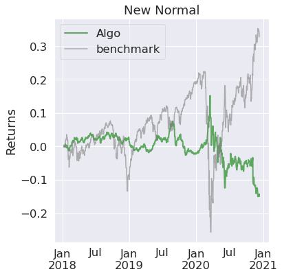
Stress Events	mean	min	max
New Normal	-0.01%	-7.48%	3.07%